There is some confusion in online video game communities about how probability works, particularly in regard to item drop chances. This seems to happen wherever players have a very low chance of obtaining something they want, and are willing to play through content repeatedly to obtain it. I’ve noticed this in Path of Exile with the Labyrinth enchantments, where there are 362 possible helmet enchantments, each with an equal probability of occuring (or a 1/362 chance of any particular enchantment occuring). This also happens in World of Warcraft (WoW), where many of the highly prized mounts have a 0.5-4% chance of dropping in a dungeon or raid playthrough.
If we had a WoW mount with a 1% chance of dropping, it is tempting to say that we simply need to run the dungeon 100 times to have a 100% chance of obtaining the mount. Many people think of probability this way, and are disappointed when it takes them many more runs through the content to finally get what they’re looking for. If the chance of something happening is 1%, or 1/100, this doesn’t guarantee that it will happen to a particular player after 100 trials. Rather, it follows the law of large numbers. Player A might find the mount after a single run, Player B after 35 runs, Player C after 500 runs, but on average, over tens or hundreds of thousands of runs, the mount will be found about once in every hundred runs.
So, how do we find our actual likelihood of finding an item (or, outcome) over a number of runs (or, trials)? I will use Deathcharger’s Reins in WoW to demonstrate. Deathcharger’s Reins is an item that drops off Baron Rivendare, the final boss of the Stratholme dungeon, and awards the ‘Rivendare’s Deathcharger’ mount. Although now owned by about 20% of players, this mount was once highly sought-after as it was the only means Alliance players had to ride an undead horse, and there are plenty of mount-collectors still looking for it. Finding this mount can be frustrating because, according to Wowhead, it drops about 0.8% of the time (or, a probability of 0.008).
Rivendare’s Deathcharger in action, being ridden by an Alliance night elf player. Image courtesy of Wowhead.

In order to find the probability, there are a couple characteristics of our ‘mount trials’ worth considering. First, the probability must always be a number between 0 and 1. A negative probability would indicate a probability that is even lower than ‘impossible’, and a probability greater than one would indicate a probability higher than ‘absolute certainty’; frankly, these values wouldn’t make any sense, and if we end up with a probability outside the 0-1 range we’ve probably done something wrong. Second, there are only two possible outcomes for every trial (either we found the mount or we didn’t), and the probability of success doesn’t change across trials. Unlike, say, the Legion legendary items, there is no ‘bad luck protection’ at play which increases the probability of success after each failure. There are no other factors, such as dungeon completion time, which can influence the drop rate of Deathcharger’s Reins off of Baron Rivendare, either.
Now, it is tempting to go for the pitfall earlier where we sum the individual probability of each run. Our equation would look something like this:
$$ P = \sum (p_{success})_n $$
Where P is our total probability, p is our probability of success on a particular run, for each n run. Or: $$ P = p(1) + p(2) + … p(n) $$
With a drop rate of 0.8%, we would need 125 runs for our added probabilities to sum to 1, or 100%. However, what if we did 126 runs? Our probability would equal 1.008. On run 127 our probability would equal 1.016. And so on. We can’t have a probability above 1, meaning we can’t sum probabilities in this way.
What if we try multiplying our probabilities? Probabilities are often multiplied when comparing events or trials. For instance, the probability of flipping a coin twice and landing on heads both times is the product of the probability of landing heads on each flip, or 0.5 * 0.5 = 0.25. Our equation would look something like this:
$$ P = (p_{success})^n $$
Our total probability is P, our probability of success for a run is p, and we have n number of runs.
If we try this over a small number of runs, we come up with another problem:
0.008 * 0.008 = 0.000064
0.008 * 0.008 * 0.008 = 0.000000512
etc.
Our probability gets smaller over a greater number of runs! If we followed this through to 125 runs like in the previous example, we would end up with an infinitesimally small probability of 7.696 * 10^-263, which may as well be 0. What we’ve actually done here is calculated the probability of success every run. So, we have a 0.8% chance of finding the mount once, a 0.0064% chance of finding the mount twice in a row, a 0.0000512% chance of finding the mount three times in a row, and so on. Unlike the previous example where we added probabilities together, this does give us useful information, but it’s not the information we’re looking for.
However, we can apply this same method to our problem, we just need to invert our thinking. Instead of working with the probability of success, we can use the probability of failure. Since our failure probability is less than 1, multiplying the failure probability for each attempt should result in an ever-decreasing number. Instead of finding the probability of success every run, we are finding the probability of failure every run. Since probability is expressed as a proportion with range 0-1, the probability of having a success over a given number of runs is the inverse of our probability of failure every run. Our equation would look something like this:
$$ P = 1 - (p_{failure})^n $$
Each run has a 0.008 probability of success (0.8%, or 1/125), so the probability of failure is 1 - 0.008 = 0.992 (or 99.2%, or 124/125) for each run. If we were to run the dungeon 125 times, what would our probability of success or failure be?
1 - (probability of failure)^number of runs
1 - (0.992)^125
1 - 0.366
0.634
In other words, after 125 runs of the Stratholme dungeon, there is a 63.4% chance we will have seen Deathcharger’s Reins drop off Baron Rivendare, and a 36.6% chance we won’t see it drop. Or perhaps more accurately, 63.4% of players should see the mount drop by time they have reached 125 runs. If we keep inputting different values for n (number of runs), it’s noticable that the relationship between number of runs and probability of success is non-linear. It takes 20 runs to reach 15%, 45 runs to reach 30%, 87 runs to reach 50%, 173 runs to reach 75%, 287 runs to reach 90%, 373 to reach 95%, 574 runs to reach 99%, 861 runs to reach 99.9%, and so on. We’ll never reach a probability of 1, except through rounding, because we can’t guarantee we’ll ever have a success (even a 50/50 coin flip can have a long streak of only-heads or only-tails if we flip enough times).
In fact, what we’re actually describing is the binomial distribution. The probability mass function of the binomial distribution describes the probability of getting a particular number of successes, given a number of attempts with unchanging independent probability of success. The probability mass function for a binomial distribution is:
$$ f(k) = \frac{n!}{k!(n-k)!} \ p^k (1-p)^{n-k} $$
Where k is the number of successes, n is the number of runs, and p is the probability of success in any particular run. The ‘!’ symbol indicates a factorial, so if n = 7, n! = 7 * 6 * 5 * 4 * 3 * 2 * 1 (since not everyone is familiar with factorials).
The binomial distribution describes the possibility of a given number of successes, rather than just one success. It’s certainly possible for us to find the Deathcharger’s Reins more than once over 125 runs. Personally I’ve seen the mount drop twice within 100 runs, and have seen other rare mounts drop in quick succession. When we found the probability of success over 125 attempts (63.4%), we were really finding the cumulative probability of having at least one success via the binomial distribution.
We can use the R language to find and graph our probabilities without too much trouble. Even though the math is fairly simple, it’s much easier and quicker to have a computer do it than to calculate by hand.
The R function dbinom() gives the probability density for a given value of k.
Probability density and probability mass (the term I used earlier) mean the same thing, but different disciplines have their own conventions and terminology.
This function takes three arguments: k, n, and p. If we set k = 0, the function returns the probability we find the mount zero times.
If we want the probability of finding the mount at least once, we invert the result:
1 - dbinom(0, 125, 0.008)This outputs ‘0.633597’, the same value (rounded to fewer digits) that we calculated by hand earlier. If we want to specify multiple values of k, we can do so, and R will give us each individual value. Here, we find the probability of finding exactly 1, 2, 3… up to 7 mounts in 125 runs.
dbinom(1:7, 125, 0.008)

# Output:
# [1] 0.3693578615 0.1846789308 0.0610631948 0.0150195762 0.0029312399
# [6] 0.0004727806 0.0000648167
Note that the sum of the outputted values is ‘0.6335883973’, very close to the ‘0.633597’ value outputted by the previous chunk of code, and to the value we calculated by hand.
We could specify greater values of k, but the probabilities become so small there’s no point in outputting them all. Instead, we can have R sum them for us and not worry about it.
Note: this returns the same result as 1 - dbinom(0, 125, 0.008):
sum(dbinom(1:125, 125, 0.008))So again, our output is ‘0.633597’. A typical player running Stratholme 125 times has a 0.634 probability, or 63.4% chance, of having the Deathcharger’s Reins drop. Now, this is fine and all, but visualizing our data can help us understand a lot more about it a lot quicker than a summed range, or heaven forbid a table of potentially hundreds of probabilities for values of k. We can use ggplot2, a visualization package (and part of the Tidyverse group of packages), to help make things more understandable. The following graphs also use theme_partywhale, a simple but clean modification of ggplot2’s theme_grey theme.
Setting y to our dbinom() probabilities, and x to the k values we want, the code for a quick binomial probability mass function is as follows:
y <- dbinom(0:10, 125, 0.008)
x <- (0:10)
qplot(x, y, colour = I("#F9858F"), size = I(4), shape = I(16)) +
  scale_x_continuous(breaks = seq(0, 10, 2)) +
  labs(title = "Binomial: Probability Mass Function",
       subtitle = "where p = 0.008 and n = 125",
       x = "Number of mount drops",
       y = "Probability") +
  theme_partywhale()
Which gives us the following graph:
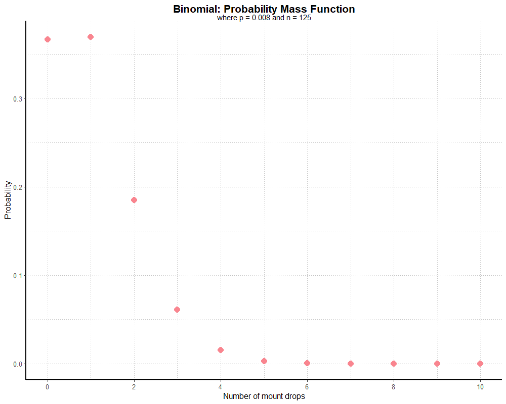
So, according to our graph, we have just over a 0.35 probability of having no mount drop, a similar probability of finding the mount exactly once, just under 0.2 probability of finding it twice, and just over 0.05 probability of finding it three times. Other values of k are so small as to be negligible (which is why I haven’t calculated all 126 possible values of k). Even without seeing the exact values, this gives us a good sense of relative probabilities for k, and with a little mental arithmetic we know our cumulative probability for k > 0 will be just over 0.6.
We can also use pbinom(), which takes the same arguments as dbinom(), to plot the
cumulative distribution function. This will give us the probability of having k or fewer successes. The equation for the cumulative distribution function is:
$$ F(k) = \sum f_i $$
And the code for our plot:
y <- pbinom(0:10, 125, 0.008)
x <- 0:10
qplot(x, y, colour = I("#F9858F"), size = I(4), shape = I(16)) +
  scale_x_continuous(breaks = seq(0, 10, 2)) +
  scale_y_continuous(breaks = seq(0.00, 1.00, 0.20)) +
  expand_limits(y = 0) +
  labs(title = "Binomial: Cumulative Distribution Function",
       subtitle = "where p = 0.008 and n = 125",
       x = "Number of mount drops",
       y = "Probability") +
  theme_partywhale()
Which gives the following graph:
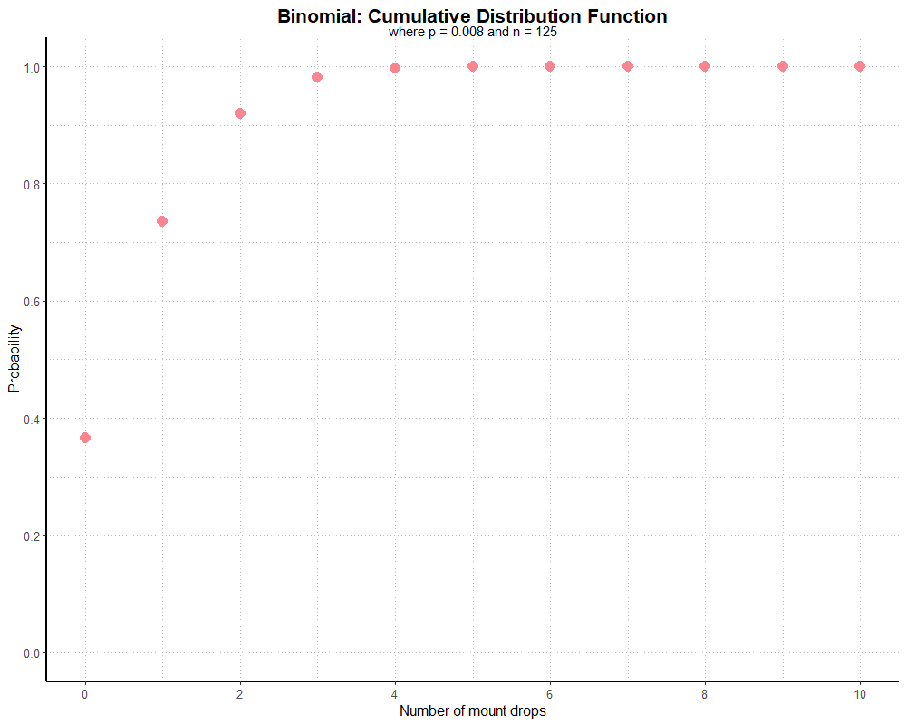
So our probability of finding 0 mounts is just over 0.35, 0-1 mounts is about 0.75, 0-2 mounts is just over 0.9, and 0-3 mounts is nearly 1. Although further values for k look like they’re at 1 on the graph, they only approach very closely to 1. If our graph went to k = 125, our probability of finding between 0 and 125 mounts over 125 runs must equal 1 (as we cannot find fewer than 0 or greater than 125). However, applied in this way, a cumulative distribution function isn’t very useful because it’s awkward to interpret. As before, we can subtract our values by one to get the probability of finding a number of mounts greater than k:
y <- pbinom(0:10, 125, 0.008, lower.tail = FALSE)
x <- 0:10
qplot(x, y, colour = I("#F9858F"), size = I(4), shape = I(16)) +
  scale_x_continuous(breaks = seq(0, 10, 2)) +
  labs(title = "Binomial: Inverse Cumulative Distribution Function",
       subtitle = "where p = 0.008 and n = 125",
       x = "Number of mount drops, greater than",
       y = "Probability") +
  theme_partywhale()
Alternatively, we could use 1 - pbinom(0:10, 125, 0.008), but R has this built-in via the lower.tail parameter. We get the following graph:
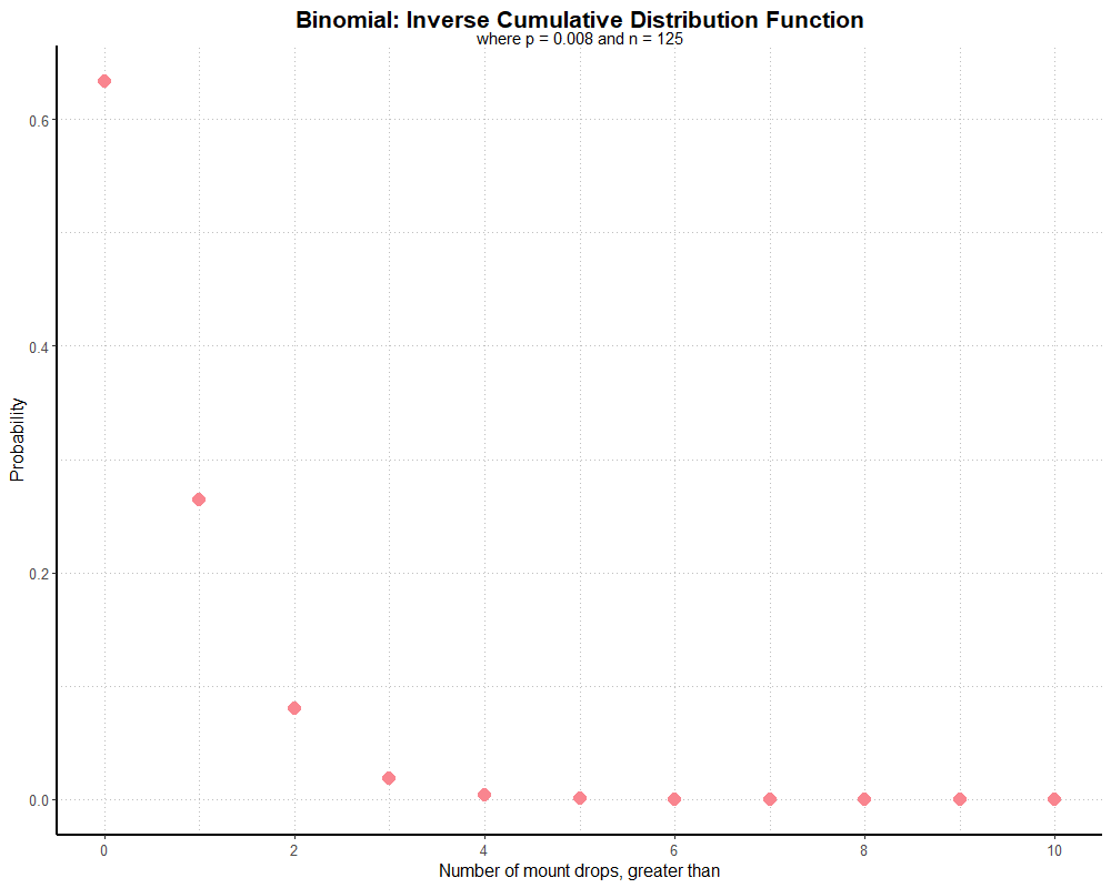
Here, the probability that we will find greater than 0 mounts (or, 1+ mounts) is just over 0.6, or 0.633597 to be exact. The probability that we will find greater than 1 mount (or, 2+ mounts) looks to be around 0.27, and so on. This graph is still a little clunky, and we would want to fix the labels (particularly on the x-axis) to make interpreting it a little easier. But, ultimately, with a little polishing this is information we can show anyone and be (reasonably) understood without having to explain a binomial distribution.
Next we’ll use simulations to test our perfect, or ‘theoretical’, binomial distributions, and take a look at the expected number of failures before a successful mount drop using the geometric distribution. But for now, this post is long enough!