In Part 1, we explored probability by calculating our chances of finding Rivendare’s Deathcharger in World of Warcraft’s Stratholme dungeon, and explored the binomial distribution. Now, we’ll use simulations to test the ‘theoretical’ distribution we generated, and take a look at the expected number of failures before a successful mount drop using the geometric distribution.
To recap, the probability mass function (PMF) for a binomial distribution is given as:
$$ f(k) = \frac{n!}{k!(n-k)!} \ p^k (1-p)^{n-k} $$
Since Rivendare’s Deathcharger (or, more specifically, the Deathcharger’s Reins items which grants this mount) drops at a rate of 0.8% (or 1/125), if we did 125 runs of the dungeon, we can find the probability of seeing the mount drop over that many runs by subtracting the PMF, where k equals 0, from 1. As it happens, we have a 63.4% chance of seeing the mount at least once over 125 dungeon runs. If we plot our probability for each potential value of k (0 through 125), we get a graph that looks like this:
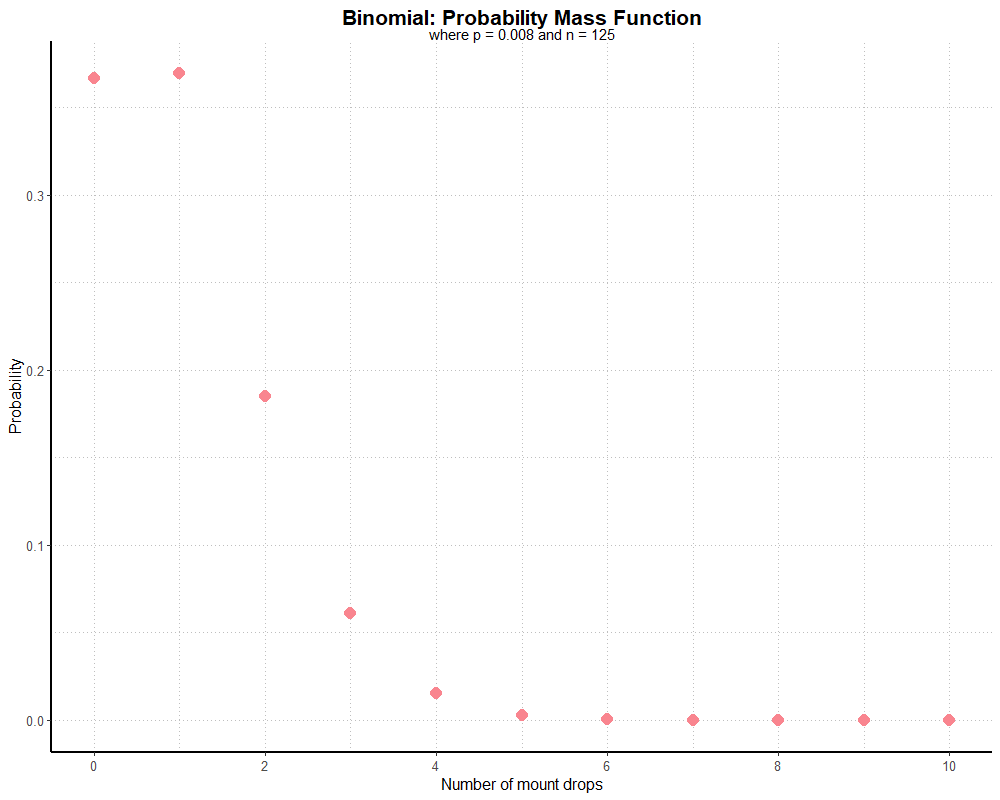
Note that this graph is truncated, as there’s little value in visualizing a distribution tail of over one hundred near-zero probabilities.
Since this graph is generated with an equation, and not actual dungeon runs, we might call it ‘theoretical’ instead of real. It’s relying on the law of large numbers; the more dungeon runs we complete, the closer a distribution based on real dungeon runs should match our theoretical one. What if we use real data?
Now, I’m not going to load up WoW and run Stratholme over and over again. I’ve done that enough in the past (Cat Druid, for speed, stealth, and AoE spam when necessary, is a good way to go about it, but you’ll hit the hourly 10 instance cap in about 40 minutes). And since the characteristics of the dungeon are known, we know the mount drop should follow a binomial distribution. From past data collection efforts, we know with reasonable certainty the drop rate is 1/125. We know there are only two outcomes, success or failure. We know the probability for each run is constant and independent, because other drop mechanics were not introduced until later parts of the game. In other words, simulating real data in this case is pretty easy. If our probability were 0.5, we could simulate dungeon runs by flipping a coin over and over again. However, we’ll have a lot of trouble finding a (real) coin that only lands on heads once every 125 flips.
If we pop open the Python shell, the random module can give us such a coin:
import random
random.randint(1, 125)
This returns an integer between (and including) 1 and 125. If we say a value of 125 is a success, we can simulate dungeon runs over and over by
repeating random.randint(1, 125). We could write a loop to repeat this line 125 times, or to keep going
until we get a value of 125. In Python 3.6 or later, we can use choices() to make this easier.
import random
sum(random.choices([0, 1], [0.992, 0.008], k = 125))
Here we define two choices, 0 for failure and 1 for success, and weight them appropriately (99.2% chance of failure, 0.8% chance of success).
Our sample size is k, set to 125, meaning we generate 125 trials. This returns a list of 125 ones and zeros.
I’m using sum() to add up the list and see how many successes we get in 125 runs (usually returning 0, 1, 2, or sometimes 3).
So, we have a customizable random number generator at our fingertips with which we can generate binomial simulations quickly, writing right into a shell!
If you remember the random module’s functions and arguments, it’s as quick as opening Windows’ calculator app.
Of course, R has this functionality built in too. The rbinom() function allows us to iterate something like our Python simulation many times:
rbinom(10, 125, 0.008)
This piece of code essentially runs 10 players through our dungeon 125 times, with a success probability of 0.008.
It’s the equivalent of running our Python code through a for loop in range(0, 9).
The output is a list with ten numbers denoting the number of successes:
1 0 2 0 0 1 1 2 0 2
So, four players didn’t see the mount drop, and 6 saw it drop at least once, which roughly corresponds with our 63.4% figure. As long as we’re not trying to run the simulation on a toaster, it’s easy to scale up, too:
rbinom(1000, 125, 0.008)Output:
1 0 2 0 1 1 1 2 0 1 0 1 1 4 1 1 1 2 2 0 0 1 0 0 2 1 0 2 1 1 0 1 0 0 1 0 0 0 1 0 0 0 2 1 0 2 0 0 5 0 0 0 1 3 0 1 0 1 1 1 0 1 0 0 0 0 1 0 0 1 0 0 2 0 0 0 3 1 0 2 1 0 2 1 2 1 1 2 1 2 1 1 2 0 0 1 3 0 0 0 0 2 1 1 0 0 1 2 2 0 0 1 2 2 2 5 1 1 1 0 1 1 1 1 2 0 0 2 2 1 0 1 1 0 1 0 1 2 1 2 0 0 2 2 1 1 1 1 3 0 2 1 0 0 4 4 1 3 0 2 0 0 1 0 0 1 2 1 0 2 1 0 0 2 1 0 2 0 0 0 1 1 3 4 1 1 0 0 1 2 1 2 1 1 1 0 0 0 2 0 0 1 1 1 1 2 1 0 0 2 2 0 0 0 0 1 1 0 1 1 0 1 1 2 0 1 1 1 1 0 2 1 2 0 2 0 1 2 1 0 2 0 1 0 0 0 1 2 1 1 0 1 1 0 1 0 1 1 1 2 1 3 0 3 0 4 1 2 0 1 1 3 1 2 1 1 1 1 3 3 0 2 0 1 0 0 2 1 0 1 2 1 0 0 2 1 1 2 0 2 1 1 1 1 0 1 1 1 3 0 2 1 2 0 0 1 3 3 4 1 1 1 1 1 0 1 0 2 1 2 1 2 1 1 1 0 3 2 0 0 4 0 2 0 0 5 0 0 0 0 1 2 0 0 2 1 1 1 0 3 0 1 1 3 2 1 0 0 2 2 4 0 1 1 0 0 4 1 0 0 2 1 1 3 1 2 1 0 1 1 4 0 3 0 3 0 0 2 1 1 1 0 1 0 2 0 1 2 1 2 1 3 0 0 1 1 1 2 0 2 1 0 2 2 2 1 0 0 0 0 1 0 1 0 2 2 0 0 1 0 1 2 1 1 0 0 2 0 0 1 0 0 2 0 0 0 1 0 1 2 0 1 2 1 0 1 0 3 1 1 2 2 1 1 2 2 0 1 1 1 0 1 1 1 0 1 2 1 0 0 1 4 1 0 0 1 1 1 1 4 1 0 2 2 0 3 1 0 0 2 1 0 0 2 0 0 1 1 0 1 2 0 1 2 1 0 0 0 0 1 0 0 1 1 1 1 2 1 1 1 3 1 2 0 0 1 2 0 1 2 0 3 1 1 0 1 2 0 1 2 1 2 1 1 0 1 2 2 1 2 1 0 2 0 3 0 1 3 0 0 1 0 1 1 2 2 0 0 2 1 0 3 2 0 1 2 0 1 2 1 1 2 0 1 2 1 0 0 3 1 3 0 3 0 1 1 1 1 0 2 0 2 2 1 1 0 0 2 0 1 1 0 0 1 0 0 3 0 1 2 0 2 0 4 0 0 0 0 1 3 0 3 0 2 0 2 0 0 0 1 2 1 0 0 2 2 1 0 2 2 1 1 1 0 1 1 1 0 1 0 0 1 0 3 1 1 1 0 2 1 1 0 1 1 1 0 0 2 0 1 2 0 0 1 2 2 2 0 1 1 1 3 0 0 0 1 1 1 0 1 2 0 1 3 1 4 1 1 2 4 1 0 1 2 3 0 1 2 0 0 3 2 1 1 1 0 1 0 2 1 1 2 2 1 3 1 1 1 0 0 2 0 0 1 0 1 0 1 0 1 0 0 1 1 1 2 2 1 2 2 0 0 0 1 0 0 0 3 3 1 0 1 1 2 0 1 0 2 3 1 0 1 2 0 2 0 0 1 1 1 0 0 1 1 3 1 1 1 0 2 0 1 2 1 0 0 1 2 0 0 0 1 1 1 1 3 1 0 0 1 1 0 0 0 1 2 1 2 1 1 0 1 1 1 0 1 2 1 1 0 1 0 1 1 2 2 0 2 2 0 1 0 0 0 2 0 2 0 1 0 2 3 1 3 1 0 1 0 2 1 0 2 0 3 1 0 1 2 1 1 0 1 1 1 2 1 0 1 0 0 3 0 0 3 0 1 1 2 0 6 0 0 2 0 1 0 0 1 2 1 1 2 1 1 0 4 3 0 1 0 1 1 2 1 0 2 2 1 3 2 0 0 0 1 3 3 0 0 2 0 1 1 1 1 1 2 0 1 1 0 0 0 0 0 2 3 2 1 1 1 0 0 2 1 0 1 1 1 1 0 0 2 2 1 0 0 0 1 1 0
Yes, that’s 1000 results of 125 trials each, or 125,000 total runs. I won’t post anymore output vomit like that, but it does demonstrate how much we can do with one line of code. Imagine what the output would look like with 100,000 samples of 125 runs (or, 12,500,000 total trials)? It would be unintelligible; also, an ideal candidate for visualization! Let’s try it:
successes <- c(as.numeric(rbinom(100000, 125, 0.008)))
id <- c(as.numeric(1:length(successes)))
df <- data.frame("id" = id, "successes" = successes)

simHistogram <- ggplot(df, aes(x = successes)) +
  geom_histogram(binwidth = 1,
                 alpha = 0.60,
                 color = "dark red",
                 aes(fill = ..count..)) +
  scale_fill_gradient("Frequency", low = "blue", high = "red") +
  labs(title = "Histogram of Number of Mount Drops",
       subtitle = "Based on 100,000 simulations of 125 dungeon runs",
       x = "Number of mount drops",
       y = "Frequency") +
  theme_partywhale()
simHistogram
This generates the following graph:
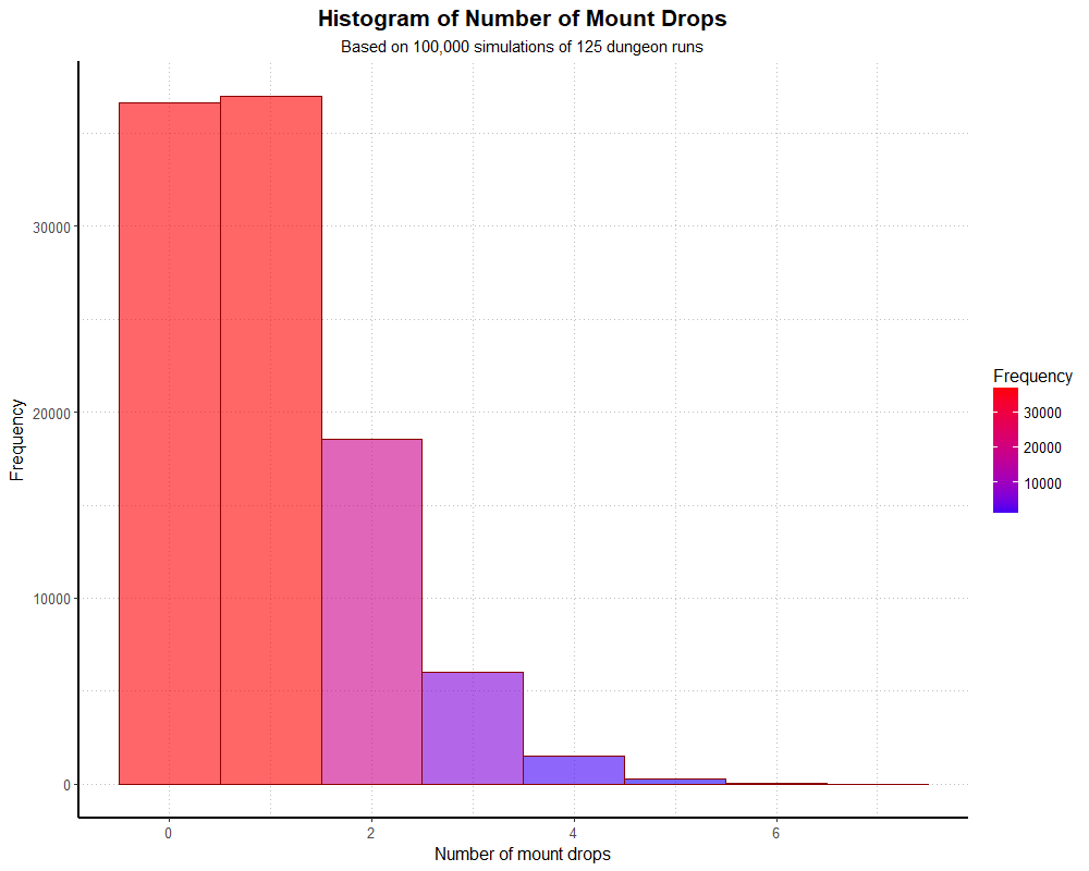
If we divide the y axis by 100,000, our simulated distribution actually matches the theoretical distribution fairly well. If we want to see a summary of the actual numbers, we can do so with a univariate frequency table.
histTable <- table(successes)
histTable
And we get:
| Number of mounts | Frequency |
|---|---|
| 0 | 36,623 |
| 1 | 37,002 |
| 2 | 18,525 |
| 3 | 6,039 |
| 4 | 1,484 |
| 5 | 286 |
| 6 | 37 |
| 7 | 4 |
In this simulation, 36.6% of players found the mount zero times after 125 runs, which matches the 36.6% we would expect from the theoretical model. We could re-run this simulation many times with different seeds, and although there will be small variations in the frequencies, we’ll end up with similar probabilities. The most noticible difference between simulations will be how far the tail reaches down the x axis.
What if, instead of simulating 100,000 players doing 125 runs each, we want to simulate 861 runs each? 861 dungeon runs is the point where the probability of seeing the mount drop at least one time reaches 99.9%. Because the overwhelming majority of players are likely to see the mount drop after 861 runs, the shape of our distribution will look different (but still follows a binomial distribution). We can generate the theoretical distribution like so:
y <- dbinom(0:20, 861, 0.008)
x <- (0:20)
df <- data.frame("id" = id, "successes" = successes)
qplot(x, y, colour = I("#F9858F"), size = I(4), shape = I(16)) +
  scale_x_continuous(breaks = seq(0, 20, 5)) +
  labs(title = "Binomial: Probability Mass Function",
       subtitle = "where p = 0.008 and n = 861",
       x = "Number of mount drops",
       y = "Probability") +
  theme_partywhale()
This generates the following graph:
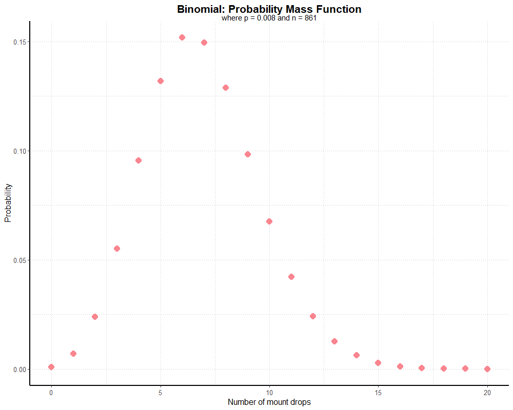
Hypothetically, the majority of players should find the mount 5-8 times over 861 runs. A very small but non-zero number of players still won’t find the mount at all.
Now, let’s simulate some dungeon runs. The code is nearly identical to our previous simulation; we just sub in a number in
the rbinom() function and a label:
successes <- c(as.numeric(rbinom(100000, 861, 0.008)))
id <- c(as.numeric(1:length(successes)))
df <- data.frame("id" = id, "successes" = successes)

simHistogram <- ggplot(df, aes(x = successes)) +
  geom_histogram(binwidth = 1,
                 alpha = 0.60,
                 color = "dark red",
                 aes(fill = ..count..)) +
  scale_fill_gradient("Frequency", low = "blue", high = "red") +
  labs(title = "Histogram of Number of Mount Drops",
       subtitle = "Based on 100,000 simulations of 861 dungeon runs",
       x = "Number of mount drops",
       y = "Frequency") +
  theme_partywhale()
simHistogram
And we get the following output:
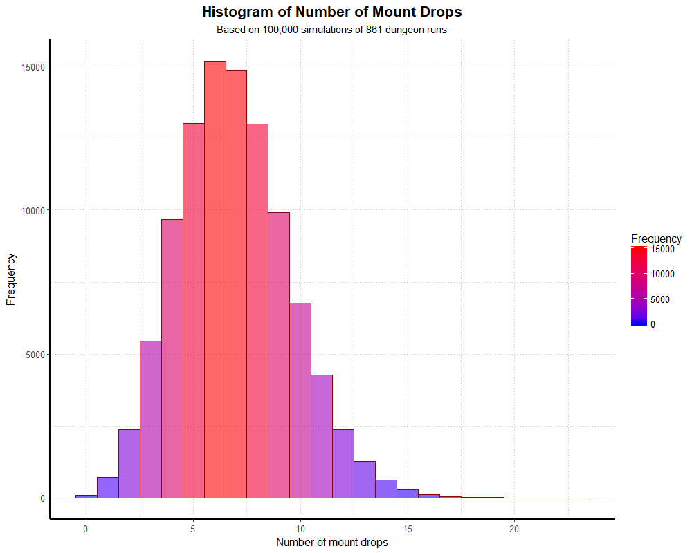
Again, dividing our frequencies by 100,000, we end up with proportions very close to the theoretical binomial distribution. We can examine the numbers with a table, as before (though I won’t print the whole thing out here).
| Number of mounts | Frequency |
|---|---|
| 0 | 92 |
| 1 | 715 |
| 2 | 2,372 |
| 3 | 5,436 |
| 4 | 9,668 |
| 5 | 13,016 |
| 6 | 15,183 |
| 7 | 14,856 |
| 8 | 12,987 |
| 9 | 9,908 |
The 0.092% of players who didn’t find the mount is pretty close to the 0.099% we would expect. With larger simulations, these should match even more closely.
One last demonstration: if we have data that follows a binomial distribution and want information on the number of failures to first success
(rather than number of successes over a set number of trials), we’ll instead be graphing a geometric distribution.
R has built-in functions for the geometric distribution as well. For our purposes, dgeom() will give us the
probability it will take a given number of failures before a success (i.e. a mount drop). For instance:
dgeom(1, 0.008)
dgeom(125, 0.008)
dgeom(300, 0.008)
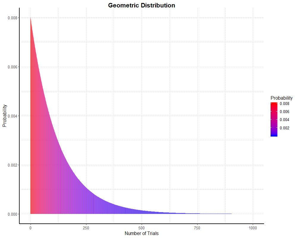
These output 0.007936, 0.002931224, and 0.0007187728 respectively. Or, 0.79% of players should find the mount on their second try, 0.29% of players on their 126th try,
and 0.072% on their 301st try. If it’s not already obvious, the probability we find the mount on our first try, or dgeom(0, 0.008),
is 0.008, our regular chance of success on any one dungeon run! We can plot a ‘theoretical’ geometric distribution with the following code (note that I’ve limited the x axis to 1000;
since a success, or in this case a mount drop, cannot be guaranteed, the x axis actually stretches to infinity).
geomSingleProb <- c(as.numeric(dgeom(0:1000, 0.008)))
dfGeomDist <- data.frame("geomSingleProb" = geomSingleProb, "x" = 0:1000)

simGeomHistogram <- ggplot(dfGeomDist, aes(x = x, y = geomSingleProb, fill = geomSingleProb, width = 1)) +
  geom_col(alpha = 0.60,
           color = NA
           ) +
  scale_fill_gradient("Probability", low = "blue", high = "red") +
  labs(title = "Geometric Distribution",
       x = "Number of Trials",
       y = "Probability") +
  theme_partywhale()
simGeomHistogram
And we get this graph:
As with the binomial examples, I’ve run a simulation to see how well real (well, simulated, but as good as real) data stacks up.
I’ve thought of two approaches here: specifying a number of players who run the dungeon until success, or specifying a blanket number of
dungeon runs and seeing how many players succeed in finding the mount. If we want to specify the number of players, we can use rgeom():
g <- rgeom(100000, 0.008)
mean(g)
median(g)
table(g)
First, I assign the rgeom() function, and take a look at some of the data it generates.
The mean is about 124 and the median about 86, which is roughly what is expected given the success probability of 1/125 and the shape of a geometric
distribution. table(g) outputs a frequency table, which demonstrates that players who require a greater number
of runs to success are represented less than those who require fewer runs. Of course, we can plot this:
gNum <- c(as.numeric(g))
df <- data.frame("gNum" = gNum)

simhist <- ggplot(df, aes(x = gNum)) +
  geom_histogram(binwidth = 1,
                 alpha = 0.60,
                 #color = "dark red",
                 aes(fill = ..count..)) +
  scale_fill_gradient("Frequency", low = "blue", high = "red") +
  labs(title = "Histogram of Number of Trials to First Success",
       subtitle = "Based on 100,000 simulations",
       x = "Trials Required",
       y = "Frequency") +
  theme_partywhale()
simhist
This outputs the following graph:
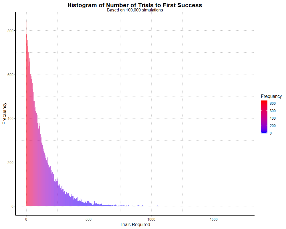
We can also find out exactly how many dungeon runs take place in this simulation (rather than number of players we specified) by summing our data,
i.e. sum(g). In this case, it comes out to roughly 12.4 million dungeon runs, which should be no surprise
given we had 100,000 players and a mean around 124 (100,000 * 124 = 12,400,000).
Now, the other way around. Let’s say we start with a set number of total dungeon runs:
p <- 0.008
trials <- runif(1e6) < p
sim <- diff(c(TRUE, which(trials)))
geomMean <- mean(sim)
geomMedian <- median(sim)
table(sim)
This specifies our probability and how many trials we want to use (1 million), resulting in a dataset similar to rgeom() without
specifying how many players are involved. I also grab the mean and median for later; in this simulation they were about 125 and 87 respectively.
Again, I looked at the frequencies with table(). Finally, I plot it, with the addition of dotted lines representing the mean and median:
simnum <- c(as.numeric(sim))
df2 <- data.frame("simnum" = simnum)

simhist <- ggplot(df2, aes(x = simnum)) +
  geom_histogram(binwidth = 1,
                 alpha = 0.60,
                 #color = "dark red",
                 aes(fill = ..count..)) +
  scale_fill_gradient("Frequency", low = "blue", high = "red") +
  geom_vline(aes(xintercept = geomMean),
             color = "deepskyblue",
             linetype = "dashed",
             size = 1) +
  geom_text(aes(geomMean, 72, label = round(geomMean, 1), hjust = -0.25), color = "deepskyblue") +
  geom_text(aes(geomMean, 75, label = "Mean", hjust = -0.30), color = "deepskyblue") +
  geom_vline(aes(xintercept=geomMedian),
             color = "darkolivegreen2",
             linetype = "dashed",
             size = 1) +
  geom_text(aes(geomMedian, 72, label = round(geomMedian, 1), hjust = 1.75), color = "darkolivegreen2") +
  geom_text(aes(geomMedian, 75, label = "Median", hjust = 1.2), color = "darkolivegreen2") +
  labs(title = "Histogram of Number of Trials to First Success",
       subtitle = "Based on 1,000,000 simulations",
       x = "Trials Required",
       y = "Frequency") +
  theme_partywhale()
simhist
This outputs the following graph:
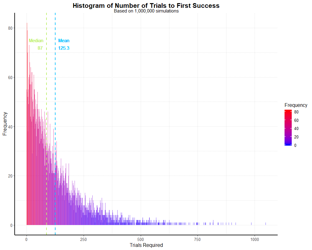
If we sum the data, i.e. sum(trials), we’ll find that this only represents 7,978 players.
As such, the graph is a little more erratic! With a larger sample, it would smooth out. We’d need to specify about 12.5 million dungeon runs for size of this
simulation to match the previous, player-based one. That said, both simulations appear to be fairly good approximations of the geometric distribution.
A note on reproducibility: since the data used in simulations are generated randomly, every time we run the simulation we will get slightly different results
(or vastly different, if we run a small simulation). Random values in R are not truly random; R uses a pseudorandom number generator utilizing the Mersenne-Twister algorithm,
which begins from a seed value. If we want to be able to reproduce a simulation exactly, we can specify a seed value at the start of our simulation
using set.seed(). For example, if I run rbinom() five times, I get five different results:
rbinom(10, 125, 0.008)
#-> 0 0 4 4 0 1 1 0 2 1
rbinom(10, 125, 0.008)
#-> 0 0 1 0 2 0 0 2 0 1
rbinom(10, 125, 0.008)
#-> 0 1 1 2 1 1 2 2 2 1
rbinom(10, 125, 0.008)
#-> 0 0 1 1 1 1 0 0 1 3
rbinom(10, 125, 0.008)
#-> 2 1 1 0 1 0 0 1 0 2
If I run rbinom() with a seed value, I will get the same result every time.
I could email the R code to someone else, and they’ll get the exact same result on their computer, too:
set.seed(1867)
rbinom(10, 125, 0.008)
#-> 0 1 0 1 1 1 0 0 1 0
I did not specify a seed when I ran the above simulations. Since the sample size is large and the data follow known distributions, this isn’t really a problem for reproducibility. Although it’s very unlikely someone else will reproduce these simulations exactly, any similarly-large simulation will arrive at values that are roughly the same. If we wanted to, we could run and record the mean of many simulations, a plot of which should be approximately normal, calculate standard deviation, and construct a confidence interval, but I’ll leave it at this for now. We’ve already learned way more than anyone should ever need to know about the Deathcharger’s Reins drop rate.